Scattering Calculations

Optical physicists and astronomers have worked out how to compute the scattering of light from many kinds of objects. HoloPy provides an easy interface for computing scattered fields, intensities, scattering matrices, cross-sections, and holograms generated by microscopic objects. (Computing scattering from macroscopic objects is computationally difficult and is not well-supported in HoloPy.)

A Simple Example

Let’s start by calculating an in-line hologram generated by a plane wave scattering from a microsphere.

import holopy as hp
from holopy.scattering import calc_holo, Sphere


sphere = Sphere(n=1.59, r=0.5, center=(4, 4, 5))

medium_index = 1.33
illum_wavelen = 0.660
illum_polarization = (1, 0)
detector = hp.detector_grid(shape=100, spacing=0.1)

holo = calc_holo(detector, sphere, medium_index, illum_wavelen,
                 illum_polarization, theory='auto')
hp.show(holo)

(Source code)

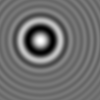
(You may need to call matplotlib.pyplot.show() if you can’t see the hologram after running this code.)

To calculate a hologram, HoloPy needs to know two things: the scatterer that is scattering the light and the experimental setup under which the hologram is recorded. With those two, HoloPy chooses an appropriate scattering theory that calculates the hologram from the scatterer and the experimental setup; advanced users may want to choose the theory themselves. We’ll examine each section of code in turn.

The first few lines :

import holopy as hp
from holopy.scattering import calc_holo, Sphere

load the relevant modules from HoloPy that we’ll need for doing our calculation.

The next line describes the scatterer we would like to model:

sphere = Sphere(n=1.59, r=0.5, center=(4, 4, 5))

Scatterers are described in HoloPy by a Scatterer object. Here, we use a Sphere as the scatterer object. A Scatterer object contains information about the geometry (position, size, shape) and optical properties (refractive index) of the object that is scattering light. We’ve defined a spherical scatterer with radius 0.5 microns and index of refraction 1.59. This refractive index is approximately that of polystyrene.

Next, we need to describe the experimental setup, including how we are illuminating our sphere, and how that light will be detected:

medium_index = 1.33
illum_wavelen = 0.66
illum_polarization = (1, 0)
detector = hp.detector_grid(shape=100, spacing=0.1)

We are going to be using red light (wavelength = 660 nm in vacuum) polarized in the x-direction to illuminate a sphere immersed in water (refractive index = 1.33). Refer to Units and Coordinate System if you’re confused about how the wavelength and polarization are specified.

The scattered light will be collected at a detector, which is frequently a digital camera mounted onto a microscope. We defined our detector as a 100 x 100 pixel array, with each square pixel of side length .1 microns. The shape argument tells HoloPy how many pixels are in the detector and affects computation time. The spacing argument tells HoloPy how far apart each pixel is. Both parameters affect the absolute size of the detector.

Finally, we need to specify the scattering theory which knows how to calculate the hologram from the experimental setup and the scatterer. By setting theory='auto', we let HoloPy automatically select a theory. If no theory is specified, HoloPy will automatically select a theory as well.

After getting everything ready, the actual scattering calculation is straightforward:

holo = calc_holo(detector, sphere, medium_index, illum_wavelen,
                 illum_polarization, theory='auto')
hp.show(holo)

Congratulations! You just calculated the in-line hologram generated at the detector plane by interference between the scattered field and the reference wave. For an in-line hologram, the reference wave is simply the part of the field that is not scattered or absorbed by the particle.

You might have noticed that our scattering calculation requires much of the same metadata we specified when loading an image. If we have an experimental image from the system we would like to model, we can use that as an argument in calc_holo() instead of our detector object created from detector_grid(). HoloPy will calculate a hologram image with pixels at the same positions as the experimental image, and so we don’t need to worry about making a detector_grid() with the correct shape and spacing arguments.

from holopy.core.io import get_example_data_path
imagepath = get_example_data_path('image0002.h5')
exp_img = hp.load(imagepath)
holo = calc_holo(exp_img, sphere)

Note that we didn’t need to explicitly specify illumination information when calling calc_holo(), since our image contained saved metadata and HoloPy used its values. Passing an image to a scattering function is particularly useful when comparing simulated data to experimental results, since we can easily recreate our experimental conditions exactly.

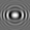
So far all of the images we have calculated are holograms, or the interference pattern that results from the superposition of a scattered wave with a reference wave. Holopy can also be used to examine scattered fields on their own. Simply replace calc_holo() with calc_field() to look at scattered electric fields (complex) or calc_intensity() to look at field amplitudes, which is the typical measurement in a light scattering experiment.

More Complex Scatterers

Let’s proceed to a few examples with different Scatterer objects. You can find a more thorough desccription of all their functionalities in the user guide on The HoloPy Scatterer.

Coated Spheres

HoloPy can also calculate holograms from coated (or multilayered) spheres. Constructing a coated sphere differs only in specifying a list of refractive indices and outer radii corresponding to the layers (starting from the core and working outwards).

coated_sphere = Sphere(center=(2.5, 5, 5), n=(1.59, 1.42), r=(0.3, 0.6))
holo = calc_holo(exp_img, coated_sphere)
hp.show(holo)

If you prefer thinking in terms of the thickness of subsequent layers, instead of their distance from the center, you can use LayeredSphere to achieve the same result:

from holopy.scattering import LayeredSphere
coated_sphere = LayeredSphere(center=(2.5, 5, 5), n=(1.59, 1.42), t=(0.3, 0.3))

Collection of Spheres

If we want to calculate a hologram from a collection of spheres, we must first define the spheres individually, and then combine them into a Spheres object:

from holopy.scattering import Spheres
s1 = Sphere(center=(5, 5, 5), n = 1.59, r = .5)
s2 = Sphere(center=(4, 4, 5), n = 1.59, r = .5)
collection = Spheres([s1, s2])
holo = calc_holo(exp_img, collection)
hp.show(holo)

Adding more spheres to the cluster is as simple as defining more sphere objects and passing a longer list of spheres to the Spheres constructor.

Non-spherical Objects

To define a non-spherical scatterer, use Spheroid or Cylinder objects. These axisymmetric scatterers are defined by two dimensions, and can describe scatterers that are elongated or squashed along one direction. By default, these objects are aligned with the z-axis, but they can be rotated into any orientation by passing a set of Euler angles to the rotation argument when defining the scatterer. See Rotations of Scatterers for information on how these angles are defined. 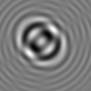As an example, here is a hologram produced by a cylinder aligned with the vertical axis (x-axis according to the HoloPy Coordinate System). Note that the hologram image is elongated in the horizontal direction since the sides of the cylinder scatter light more than the ends.

import numpy as np
from holopy.scattering import Cylinder
c = Cylinder(center=(5, 5, 7), n = 1.59, d=0.75, h=2, rotation=(0,np.pi/2, 0))
holo = calc_holo(exp_img, c)
hp.show(holo)

More Complex Experimental Setups

While the examples above will be sufficient for most purposes, there are a few additional options that are useful in certain scenarios.

Multi-channel Holograms

Sometimes a hologram may include data from multiple illumination sources, such as two separate wavelengths of incident light. In this case, the extra arguments can be passed in as a dictionary object, with keys corresponding to dimension names in the image. You can also use a multi-channel experimental image in place of calling detector_grid().

illum_dim = {'illumination':['red', 'green']}
n_dict = {'red':1.58,'green':1.60}
wl_dict = {'red':0.690,'green':0.520}
det_c = hp.detector_grid(shape=200, spacing=0.1, extra_dims = illum_dim)
s_c = Sphere(r=0.6, n=n_dict, center=[6,6,6])
holo = calc_holo(det_c, s_c, illum_wavelen=wl_dict, illum_polarization=(0,1), medium_index=1.33)

Scattering Theories in HoloPy

HoloPy contains a number of scattering theories to model the scattering from different kinds of scatterers. You can specifiy a scattering theory by setting the theory keyword to a ScatteringTheory object, rather than setting the theory to 'auto'. For instance, to force HoloPy to calculate the hologram of a sphere using Mie theory (the theory which exactly describes scattering from a spherical particle), we set the theory keyword to an instance of the Mie class:

from holopy.scattering.theory import Mie
theory = Mie()
holo = calc_holo(detector, sphere, medium_index, illum_wavelen,
                 illum_polarization, theory=theory)

HoloPy has multiple scattering theories which work for different types of scatterers and which describe particle scattering and interactions with the optical train in varying degrees of complexity. HoloPy has scattering theories that describe scattering from individual spheres, layered spheres, clusters of spheres, spheroids, cylinders, and arbitrary objects. Some of these scattering theories can take parameters to modify how the theory performs the calculation (by, e.g., making certain approximations or specifying properties of the optical train). For a more thorough description of these scattering theories and how HoloPy chooses default scattering theories, see the user guide, The HoloPy Scattering Theories.

Detector Types in HoloPy

The detector_grid() function we saw earlier creates holograms that display nicely and are easily compared to experimental images. However, they can be computationally expensive, as they require calculations of the electric field at many points. If you only need to calculate values at a few points, or if your points of interest are not arranged in a 2D grid, you can use detector_points(), which accepts either a dictionary of coordinates or indvidual coordinate dimensions:

x = [0, 1, 0, 1, 2]
y = [0, 0, 1, 1, 1]
z = -1
coord_dict = {'x': x, 'y': y, 'z': z}
detector = hp.detector_points(x = x, y = y, z = z)
detector = hp.detector_points(coord_dict)

The coordinates for detector_points() can be specified in terms of either Cartesian or spherical coordinates. If spherical coordinates are used, the center value of your scatterer is ignored and the coordinates are interpreted as being relative to the scatterer.

Static light scattering calculations

Scattering Matrices

In a static light scattering measurement you record the scattered intensity at a number of locations. A common experimental setup contains multiple detectors at a constant radial distance from a sample (or a single detector on a goniometer arm that can swing to multiple angles.) In this kind of experiment you are usually assuming that the detector is far enough away from the particles that the far-field approximation is valid, and you are usually not interested in the exact distance of the detector from the particles. So, it’s most convenient to work with amplitude scattering matrices that are angle-dependent. (See [Bohren1983] for further mathematical description.)

import numpy as np
from holopy.scattering import calc_scat_matrix

detector = hp.detector_points(theta = np.linspace(0, np.pi, 100), phi = 0)
distant_sphere = Sphere(r=0.5, n=1.59)
matr = calc_scat_matrix(detector, distant_sphere, medium_index, illum_wavelen)

Here we omit specifying the location (center) of the scatterer. This is only valid when you’re calculating a far-field quantity. Similarly, note that our detector, defined from a detector_points() function, includes information about direction but not distance. It is typical to look at scattering matrices on a semilog plot. You can make one as follows:

import matplotlib.pyplot as plt
plt.figure()
plt.semilogy(np.linspace(0, np.pi, 100), abs(matr[:,0,0])**2)
plt.semilogy(np.linspace(0, np.pi, 100), abs(matr[:,1,1])**2)
plt.show()

(Source code)

You are usually interested in the intensities of the scattered fields, which are proportional to the modulus squared of the amplitude scattering matrix. The diagonal elements give the intensities for the incident light and the scattered light both polarized parallel and perpendicular to the scattering plane, respectively.

Scattering Cross-Sections

The scattering cross section provides a measure of how much light from an incident beam is scattered by a particular scatterer. Similar to calculating scattering matrices, we can omit the position of the scatterer for calculation of cross sections. Since cross sections integrates over all angles, we can also omit the detector argument entirely:

from holopy.scattering import calc_cross_sections
x_sec = calc_cross_sections(distant_sphere, medium_index, illum_wavelen, illum_polarization)

x_sec returns an array containing four elements. The first element is the scattering cross section, specified in terms of the same units as wavelength and particle size. The second and third elements are the absorption and extinction cross sections, respectively. The final element is the average value of the cosine of the scattering angle.